Why “high accuracy” can still hide serious mistakes
A model can report 97% accuracy and still be dangerous, because “accuracy” averages over everything you chose to count. If 97 out of 100 images are easy, the model can ace them and still fail on the three that matter: the blurry badge at a security gate, the hairline crack on a part, the unusual lighting in a store aisle. Those rare cases are often the ones tied to safety, fraud, or cost.
High accuracy also hides where the model is confident but wrong. Vision models learn shortcuts—backgrounds, camera angles, timestamps, even hospital-specific markers—that correlate with labels in training data. When those cues change in the real world, the model can keep sounding sure while drifting into silent errors, and the bill shows up later in escalations, rework, or missed incidents.
The most common hidden error patterns in vision models
You’ll usually see the same failure shapes repeated across domains. The first is “shortcut learning”: the model predicts the label from an incidental cue, like a specific background, barcode placement, surgical drape color, or a store’s lighting pattern. It looks great in validation, then breaks when the cue disappears.
A second is “coverage gaps” that don’t show up in top-line metrics: certain shifts, skin tones, materials, product revisions, camera models, or night conditions are rare in training but common enough in production to cause steady loss. A third is “boundary confusion,” where near-miss classes get swapped—scratch vs. crack, benign vs. malignant-looking, employee badge vs. visitor badge—often with high confidence.
Finally, there’s “confidence inflation.” Many vision systems output probabilities that are poorly calibrated, so 0.95 doesn’t mean “right 95% of the time.” Fixing this isn’t free: you need targeted data collection, slice-level evaluation, and human review time to uncover where these patterns cluster.
Where the errors come from: data, labels, and objectives
A lot of “mysterious” vision failures come from ordinary data decisions. If training images mostly come from one factory line, one store layout, one hospital system, or one phone camera generation, the model learns that world. Even when you add more data, the long tail is expensive: rare defects, night scenes, unusual body positions, and new packaging versions don’t show up often unless someone actively hunts for them and budgets for new collection.
Labels are the next leak. In many pipelines, labels are produced under time pressure with vague guidelines, inconsistent annotators, or missing context (one frame of a video, one view of a part). That creates “soft” ground truth where the model is punished for the wrong reasons and later becomes confidently wrong on exactly the ambiguous cases humans disagree about.
Objectives quietly steer behavior too. Optimizing overall accuracy (or a single loss) encourages the model to win on the majority class, not to be cautious on high-cost errors. If missing one crack costs more than flagging ten false alarms, the training target needs to reflect that trade-off.
How to detect hidden errors before they hit production
A familiar warning sign is when a model looks stable in offline validation, but small operational changes make the outputs swing: a new camera mount, a firmware update, a different shift’s lighting, a new supplier’s materials. Before deployment, replay those “almost the same, but not quite” conditions on purpose. Build a stress set with targeted variations—crop tighter, add motion blur, change exposure, rotate, occlude key regions—and compare not just accuracy, but what it gets wrong and how confident it is when it’s wrong.
Slice analysis is the fastest way to turn vague risk into a concrete list. Break results down by site, device, time of day, product revision, patient cohort, or any metadata you actually have. Then add “model-driven” slices: clusters of high-confidence errors, near-boundary predictions, and examples where similar images get different labels. A few dozen carefully reviewed failures can reveal a shortcut cue or a missing coverage pocket.
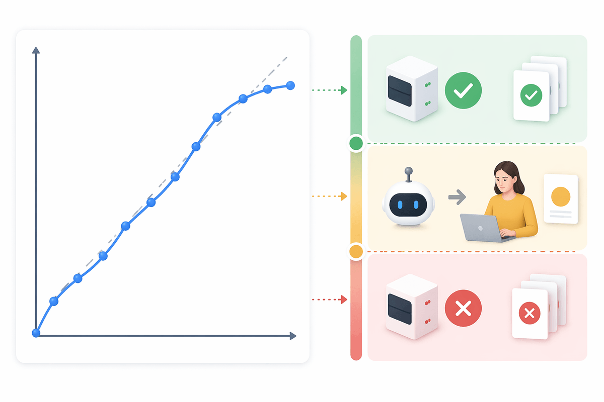
Calibration checks make confidence usable for operations. Plot reliability curves and track error rates at confidence thresholds you plan to automate on (for example, “auto-accept above 0.98”). You’ll need human review time, agreed labeling guidelines, and a tight loop to feed discovered edge cases back into the test set—otherwise the same silent failures return under a new form.
Choosing metrics that expose risk, not just performance
A common trap is choosing a metric because it’s easy to report, not because it matches the business risk. Overall accuracy or mean average precision can look strong while the model still misses the rare “stop-the-line” defect, or confidently approves a risky badge at a gate. Start by naming the costly failures, then measure them directly: per-class recall for “must-catch” classes, false accept rate at a fixed operating threshold, and performance at the top end of confidence where you plan to automate.
Bring cost into the metric rather than arguing about it later. Use weighted error rates (or explicit cost matrices) so one miss can count like ten false alarms if that reflects reality. For detection and segmentation, track worst-slice performance and not just the average—minimum recall across sites or devices often predicts production pain better than global scores.
Track calibration error and “error-at-confidence” curves (for example, the observed error rate among predictions above 0.99). The limitation is practical: many of these metrics need enough edge-case volume and consistent labeling to be statistically stable, which means budgeting for targeted data collection and review.
Reducing hidden errors: fixes that actually move the needle

The fixes that matter tend to look boring: collect the right data, fix labels, and force the model to learn the right signal. Start with a “closed loop” around your top failure slices. Pull recent high-confidence errors and near-misses from each site/device, label them with tighter guidelines (and a clear “ambiguous” option), then add them to a locked stress set you rerun every training cycle. If the model improves on average but regresses on that set, treat it as a release blocker.
When shortcut cues drive failures, try interventions that break the correlation instead of hoping more data will. Crop to the region of interest, mask known spurious areas (backgrounds, timestamps, rulers), or add counterexamples where the shortcut is present without the label. If the business cost is asymmetric, train with cost-sensitive losses or sampling so “must-catch” cases get extra weight, then calibrate and set a high-automation threshold with a human-review band in the middle.
None of this is free. Targeted collection and relabeling take time, and reviewers need training and audits. The payoff is that you stop chasing global accuracy and start buying down specific, repeatable risks.
Monitoring in the real world: drift, feedback, and guardrails
The first week after launch often looks fine, then the world moves. A camera gets cleaned, a lens is swapped, a supplier changes a finish, a store remodel shifts backgrounds, a hospital adds a new overlay. The model may not fail loudly; it can just slide into “confidently wrong.” Monitor input and output signals that correlate with risk: image quality stats (blur, exposure), embedding-distance or anomaly scores for “unfamiliar” images, and the rate of high-confidence predictions in each key slice (site, device, shift, product revision).
Set up feedback that you can actually sustain. Sample for review by risk, not randomly: high-confidence accepts, near-threshold cases, and new or fast-changing slices. Track disagreement rates between annotators and the model; spikes often mean drift or unclear labeling. Budget matters here: review time and ground truth lag are the bottleneck, so pick small, repeatable audits over one-off “big” relabel efforts.
Guardrails turn monitoring into action. Use three lanes: auto-approve only above a proven confidence threshold, auto-reject where false accepts are unacceptable, and route the middle band (plus anomaly hits) to humans. Add rate limits and kill switches by slice so one bad camera or one new SKU can’t quietly dominate decisions, and require your locked stress set to pass before any retrain goes live.
A practical way to think about “reliability” for image recognition
In practice, “reliability” is the ability to predict failure, not just to reduce it. A reliable vision model behaves like a controlled process: you know which slices it’s safe to automate, what confidence actually buys you, and how quickly you’ll notice when conditions change. The right question becomes “What percent of decisions are both accurate and appropriately routed?”—auto-approved when the error cost is low, escalated when uncertainty or novelty is high, and blocked when the risk is unacceptable.
That framing forces concrete commitments: a locked stress set that represents your real risk, operating thresholds tied to observed error-at-confidence, and slice-level guardrails that can shut down automation when drift shows up. The constraint is organizational, not mathematical: reliability requires ongoing review capacity, stable labeling rules, and the willingness to slow down releases when the risk signals degrade.